04.4.1 应用的基本条件
在临床研究中,混杂偏倚(Confounding Bias)是阻碍我们发现真实因果关系的重大障碍。在构建“双维融合的精准分层诊疗体系”中,针对患者群体的不同预后特征(如肿瘤分期、年龄分段等)进行分层卡方检验(Cochran-Mantel-Haenszel 检验,CMH 检验),可以帮助我们剥离混杂偏倚,看清治疗方案的“本质疗效”。
CMH 检验主要用于分析两个二分类变量(自变量与因变量)之间的关联性,同时控制一个或多个分类混杂因素的影响。
A. 必须满足的基本条件
观测独立性:每个患者只能归属于交叉表中的一个格子(无重复计数)。
变量属性:
自变量为二分类(如:治疗A组 / 治疗B组)。
因变量为二分类(如:无复发 / 复发)。
分层混杂变量为分类变量(如:临床I期 / 临床II期)。
样本量要求:各分层内的 2×2 交叉表总样本量不宜过小(建议各层 N ≥40)。
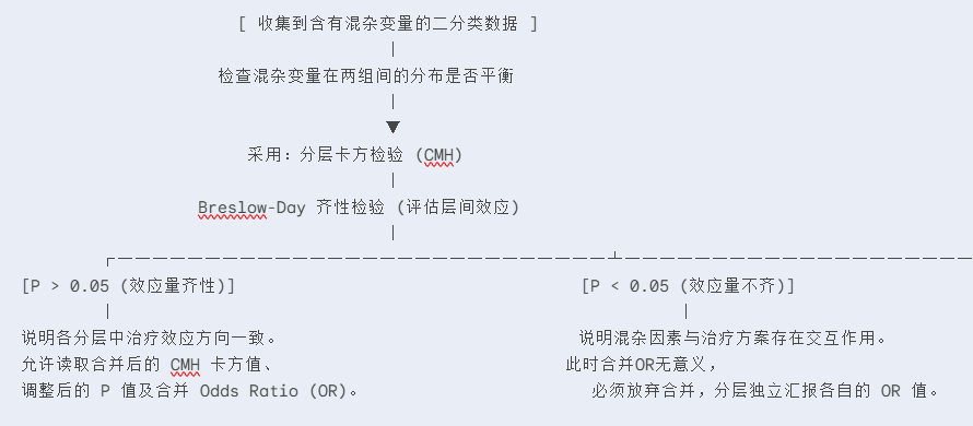
B. 满足条件的正面示例:
研究背景:在“双维融合的精准分层诊疗体系”中,研究团队拟评价两套靶向维持治疗方案(方案A vs 方案B)对非小细胞肺癌(NSCLC)患者1年无复发状态(无复发/复发)的实际效果。
数据情况:由于入组患者包含“早期(临床I期)”与“进展期(临床II期)”两类群体,且两组间分期比例分布不均(分期会同时影响方案选择和复发结局,属于典型的分类混杂因素)。自变量(方案)为二分类,因变量(复发转归)为二分类,分层变量(分期)为二分类。
判定:完全符合 CMH 检验的应用条件,可通过分层消除分期带来的混杂干扰。
C. 不满足条件的负面示例(因果剖析与统计取舍):
在实际临床分析中,如果混杂因素不具备分类特征或样本结构不合理,强行套用 CMH 检验将导致严重错误:
反面案例 1:混杂因素为连续性变量(如:年龄、连续的生物标志物浓度)
研究背景:评估新药与老药对患者1年存活率(生存/死亡)的差异,需要控制患者的连续年龄(如20-80岁,未分组)这一混杂因素。
错用因果:CMH 检验只能处理分类分层。如果将未分组的连续年龄直接作为分层变量,SPSS 会将每一个具体的年龄值(如 41岁、42岁、43岁...)强制识别为一个独立的层,从而产生几十个极度稀疏的“空壳层”。每一层内仅包含 1-2 例受试者,导致卡方公式在计算期望频数时分母趋近于零,系统报错或估算出的 OR 值产生严重偏倚(失真)。
取舍策略:
方案一(推荐):放弃分层卡方,直接采用二元 Logistic 回归(Binary Logistic Regression),将药物分组(分类)和连续年龄(协变量)同时纳入模型进行多因素校正。
方案二:根据临床指南将年龄转化为等级分类变量(如:<60岁为中青年组,≥60岁为老年组),再采用标准 CMH 检验。
反面案例 2:小样本下过度分层(导致多层内出现零细胞,即“稀疏数据”)
研究背景:在一项小样本(N = 45)的临床探索性试验中,对比两组患者的疗效(有效/无效)。研究者为了追求完美,试图同时控制“性别(2层)”、“肿瘤病理类型(3层)”和“吸烟史(2层)”三个混杂因素。
错用因果:CMH 的分层总数等于所有分层水平的乘积。本例的分层总数为 2×3×2 = 12层。45 例患者被分配到 12 个分层后,平均每层只有不到 4 人。进入 2×2列表后,大部分格子的人数和理论频数都变为了 0。此时不仅 Breslow-Day 齐性检验由于方差不齐无法运行,CMH 加权算法也会因为大量格子频数为 0 导致加权权重失效,无法得出可信的合并 OR。
取舍策略:
方案一:合并或精简分层。在不违背临床专业逻辑的前提下,只保留最核心的一个分类混杂因素(如仅保留病理类型),删除或忽略次要混杂,使每层内样本充盈。
方案二:如果样本量确实无法增加,应采用精确 Logistic 回归(Exact Logistic Regression)或使用 Firth 惩罚最大似然估计进行多因素校正,而非强行分层。
04.4.2 核心概念深度剖析:为什么必须控制混杂?
A. 什么是混杂?
假设在总体数据中,治疗A组的无复发率显著高于治疗B组。但深入分析后发现,治疗A组里分配了大量的“临床I期(预后极好)”受试者,而治疗B组里大部分是“临床II期(预后极差)”受试者。 此时,“临床分期”同时影响了患者的方案选择和临床转归,这就是混杂偏倚。直接合并算出的 P 值和 OR值会产生虚假的放大或缩小。
B. 辛普森悖论(Simpson's Paradox)
这是医学统计中最著名的“视觉魔术”:在分层分析时,每个分层中都是方案 A 优于方案 B;但是一旦把所有层的数据简单粗暴地合并到一起,竟然得出了方案 B 优于方案 A 的相反结论。这就是不加控制的混杂偏倚导致的统计学灾难。
C. CMH 检验的解决方案
CMH 检验在后台分别计算每个层(Stratum)的卡方值、实际频数和理论频数,最后通过加权合并的方式,计算出一个排除分层干扰的加权合并 OR值(Common Odds Ratio)。
04.4.3 SPSS实战案例
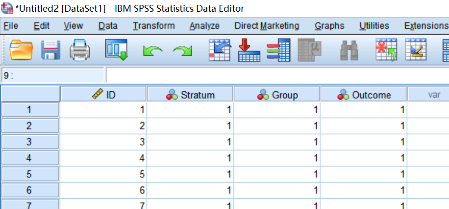
A. 数据录入
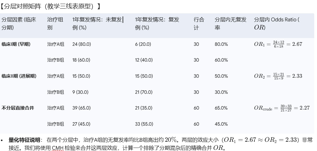
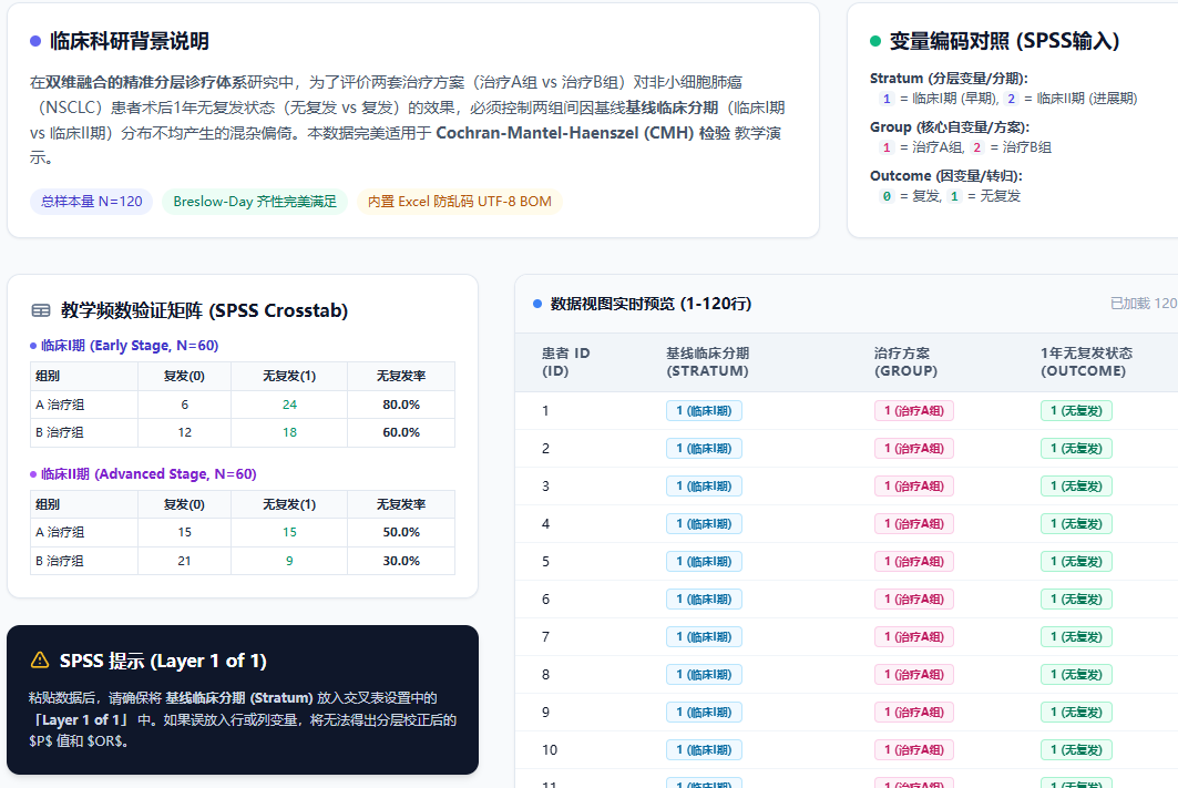
第一步:数据录入
第二步:进入交叉表多层模块
点击顶部菜单:分析 (Analyze) ──► 描述统计 (Descriptive Statistics) ──► 交叉表 (Crosstabs...)。
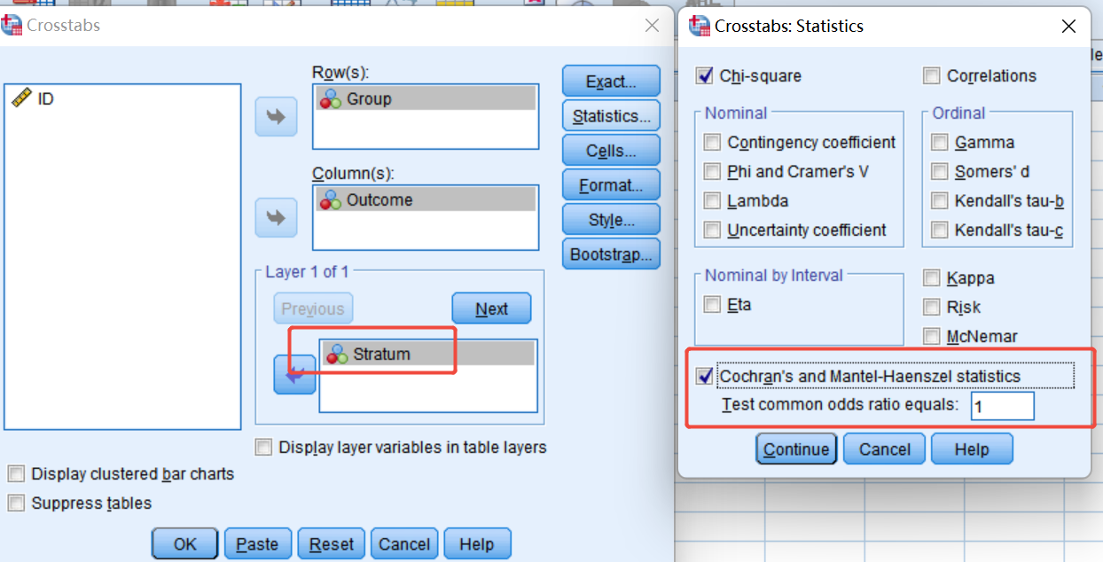
变量多维布局(核心教学点:Layer 的使用)
将 治疗方案 Group(自变量)选入 行 (Row) 框中。
将 1年无复发状态 Outcome(因变量)选入 列 (Column) 框中。
【分层核心】 将 基线临床分期Stratum(分层混杂变量)选入 层 1 (Layer 1 of 1) 框中。
第三步:勾选 CMH 统计量,设置百分比与运行
点击右侧 “统计 (Statistics...)” 按钮。
勾选 卡方 (Chi-square)。
【核心动作】 勾选最下方的 Cochran's 和 Mantel-Haenszel 统计量 (Cochran's and Mantel-Haenszel statistics)。
在其右侧自动激活的 检验公共几率比为 (Test common odds ratio equals) 输入框中,保持默认数值 1 即可。
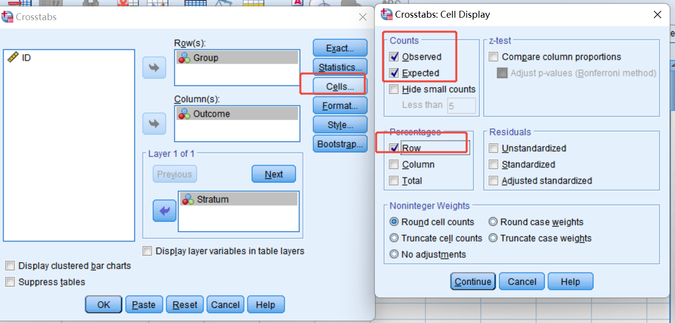
点击右侧 “单元格 (Cells...)” 按钮。
在“百分比 (Percentages)”中,勾选 行 (Row)。
点击 继续 (Continue),再点击 确定 (OK)。
04.4.4 结果解读与论文汇报规范
A. 频数表与卡方检验表
运行后,SPSS 输出结果除了给出“每个分层单独的普通卡方表格”外,最重要的是给出了以下两张判定整体疗效的灵魂表格:
| Group * Outcome * Stratum Crosstabulation | Group * Outcome * Stratum Crosstabulation | Group * Outcome * Stratum Crosstabulation | Group * Outcome * Stratum Crosstabulation | Group * Outcome * Stratum Crosstabulation | Group * Outcome * Stratum Crosstabulation | Group * Outcome * Stratum Crosstabulation |
|---|---|---|---|---|---|---|
| Stratum | Stratum | Stratum | Stratum | Outcome | Outcome | Total |
| Stratum | Stratum | Stratum | Stratum | 0 | 1 | Total |
| 1 | Group | 1 | Count | 6 | 24 | 30 |
| 1 | Group | 1 | Expected Count | 9.0 | 21.0 | 30.0 |
| 1 | Group | 1 | % within Group | 20.0% | 80.0% | 100.0% |
| 1 | Group | 2 | Count | 12 | 18 | 30 |
| 1 | Group | 2 | Expected Count | 9.0 | 21.0 | 30.0 |
| 1 | Group | 2 | % within Group | 40.0% | 60.0% | 100.0% |
| 1 | Total | Total | Count | 18 | 42 | 60 |
| 1 | Total | Total | Expected Count | 18.0 | 42.0 | 60.0 |
| 1 | Total | Total | % within Group | 30.0% | 70.0% | 100.0% |
| 2 | Group | 1 | Count | 15 | 15 | 30 |
| 2 | Group | 1 | Expected Count | 18.0 | 12.0 | 30.0 |
| 2 | Group | 1 | % within Group | 50.0% | 50.0% | 100.0% |
| 2 | Group | 2 | Count | 21 | 9 | 30 |
| 2 | Group | 2 | Expected Count | 18.0 | 12.0 | 30.0 |
| 2 | Group | 2 | % within Group | 70.0% | 30.0% | 100.0% |
| 2 | Total | Total | Count | 36 | 24 | 60 |
| 2 | Total | Total | Expected Count | 36.0 | 24.0 | 60.0 |
| 2 | Total | Total | % within Group | 60.0% | 40.0% | 100.0% |
| Total | Group | 1 | Count | 21 | 39 | 60 |
| Total | Group | 1 | Expected Count | 27.0 | 33.0 | 60.0 |
| Total | Group | 1 | % within Group | 35.0% | 65.0% | 100.0% |
| Total | Group | 2 | Count | 33 | 27 | 60 |
| Total | Group | 2 | Expected Count | 27.0 | 33.0 | 60.0 |
| Total | Group | 2 | % within Group | 55.0% | 45.0% | 100.0% |
| Total | Total | Total | Count | 54 | 66 | 120 |
| Total | Total | Total | Expected Count | 54.0 | 66.0 | 120.0 |
| Total | Total | Total | % within Group | 45.0% | 55.0% | 100.0% |
| Chi-Square Tests | Chi-Square Tests | Chi-Square Tests | Chi-Square Tests | Chi-Square Tests | Chi-Square Tests | Chi-Square Tests |
|---|---|---|---|---|---|---|
| Stratum | Stratum | Value | df | Asymptotic Significance (2-sided) | Exact Sig. (2-sided) | Exact Sig. (1-sided) |
| 1 | Pearson Chi-Square | 2.857c | 1 | .091 | ||
| 1 | Continuity Correctionb | 1.984 | 1 | .159 | ||
| 1 | Likelihood Ratio | 2.899 | 1 | .089 | ||
| 1 | Fisher's Exact Test | .158 | .079 | |||
| 1 | Linear-by-Linear Association | 2.810 | 1 | .094 | ||
| 1 | N of Valid Cases | 60 | ||||
| 2 | Pearson Chi-Square | 2.500d | 1 | .114 | ||
| 2 | Continuity Correctionb | 1.736 | 1 | .188 | ||
| 2 | Likelihood Ratio | 2.521 | 1 | .112 | ||
| 2 | Fisher's Exact Test | .187 | .094 | |||
| 2 | Linear-by-Linear Association | 2.458 | 1 | .117 | ||
| 2 | N of Valid Cases | 60 | ||||
| Total | Pearson Chi-Square | 4.848a | 1 | .028 | ||
| Total | Continuity Correctionb | 4.074 | 1 | .044 | ||
| Total | Likelihood Ratio | 4.883 | 1 | .027 | ||
| Total | Fisher's Exact Test | .043 | .022 | |||
| Total | Linear-by-Linear Association | 4.808 | 1 | .028 | ||
| Total | N of Valid Cases | 120 | ||||
| a. 0 cells (0.0%) have expected count less than 5. The minimum expected count is 27.00. | a. 0 cells (0.0%) have expected count less than 5. The minimum expected count is 27.00. | a. 0 cells (0.0%) have expected count less than 5. The minimum expected count is 27.00. | a. 0 cells (0.0%) have expected count less than 5. The minimum expected count is 27.00. | a. 0 cells (0.0%) have expected count less than 5. The minimum expected count is 27.00. | a. 0 cells (0.0%) have expected count less than 5. The minimum expected count is 27.00. | a. 0 cells (0.0%) have expected count less than 5. The minimum expected count is 27.00. |
| b. Computed only for a 2x2 table | b. Computed only for a 2x2 table | b. Computed only for a 2x2 table | b. Computed only for a 2x2 table | b. Computed only for a 2x2 table | b. Computed only for a 2x2 table | b. Computed only for a 2x2 table |
| c. 0 cells (0.0%) have expected count less than 5. The minimum expected count is 9.00. | c. 0 cells (0.0%) have expected count less than 5. The minimum expected count is 9.00. | c. 0 cells (0.0%) have expected count less than 5. The minimum expected count is 9.00. | c. 0 cells (0.0%) have expected count less than 5. The minimum expected count is 9.00. | c. 0 cells (0.0%) have expected count less than 5. The minimum expected count is 9.00. | c. 0 cells (0.0%) have expected count less than 5. The minimum expected count is 9.00. | c. 0 cells (0.0%) have expected count less than 5. The minimum expected count is 9.00. |
| d. 0 cells (0.0%) have expected count less than 5. The minimum expected count is 12.00. | d. 0 cells (0.0%) have expected count less than 5. The minimum expected count is 12.00. | d. 0 cells (0.0%) have expected count less than 5. The minimum expected count is 12.00. | d. 0 cells (0.0%) have expected count less than 5. The minimum expected count is 12.00. | d. 0 cells (0.0%) have expected count less than 5. The minimum expected count is 12.00. | d. 0 cells (0.0%) have expected count less than 5. The minimum expected count is 12.00. | d. 0 cells (0.0%) have expected count less than 5. The minimum expected count is 12.00. |
B. 层间几率比均一性检验(Breslow-Day 齐性检验)
这是我们在解读 CMH 前必须通过的“预检验”。
| Tests of Homogeneity of the Odds Ratio | Tests of Homogeneity of the Odds Ratio | Tests of Homogeneity of the Odds Ratio | Tests of Homogeneity of the Odds Ratio |
|---|---|---|---|
| Chi-Squared | df | Asymptotic Significance (2-sided) | |
| Breslow-Day | .028 | 1 | .867 |
| Tarone's | .028 | 1 | .867 |
🎯 读表决策要领(核心教学点):
读取 Breslow-Day 的 P值:本案例中 P = 0.867 > 0.05。
统计学意义:这证明两层(早期和进展期)中的治疗效应大小(即两层的 OR值 2.67 与 2.33)是同质、无显著差异的(Homogeneous)。
下阶段动作:既然两层效应方向和大小高度一致,允许我们合并这两层的数据,直接进入下一步读取合并后的 CMH 疗效。
(避坑:如果 Breslow-Day 的 P < 0.05,代表临床分期 and 治疗方案之间存在强烈的交互作用,合并OR毫无意义,必须分别独立汇报早期 and 进展期的不同疗效。)
Mantel-Haenszel 统计量与合并效应量(合并 OR估算)
| Tests of Conditional Independence(独立性检验) | Tests of Conditional Independence(独立性检验) | Tests of Conditional Independence(独立性检验) | Tests of Conditional Independence(独立性检验) |
|---|---|---|---|
| Chi-Squared | df | Asymptotic Significance (2-sided) | |
| Cochran's | 5.333 | 1 | .021 |
| Mantel-Haenszel | 4.407 | 1 | .036 |
| Under the conditional independence assumption, Cochran's statistic is asymptotically distributed as a 1 df chi-squared distribution, only if the number of strata is fixed, while the Mantel-Haenszel statistic is always asymptotically distributed as a 1 df chi-squared distribution. Note that the continuity correction is removed from the Mantel-Haenszel statistic when the sum of the differences between the observed and the expected is 0. | Under the conditional independence assumption, Cochran's statistic is asymptotically distributed as a 1 df chi-squared distribution, only if the number of strata is fixed, while the Mantel-Haenszel statistic is always asymptotically distributed as a 1 df chi-squared distribution. Note that the continuity correction is removed from the Mantel-Haenszel statistic when the sum of the differences between the observed and the expected is 0. | Under the conditional independence assumption, Cochran's statistic is asymptotically distributed as a 1 df chi-squared distribution, only if the number of strata is fixed, while the Mantel-Haenszel statistic is always asymptotically distributed as a 1 df chi-squared distribution. Note that the continuity correction is removed from the Mantel-Haenszel statistic when the sum of the differences between the observed and the expected is 0. | Under the conditional independence assumption, Cochran's statistic is asymptotically distributed as a 1 df chi-squared distribution, only if the number of strata is fixed, while the Mantel-Haenszel statistic is always asymptotically distributed as a 1 df chi-squared distribution. Note that the continuity correction is removed from the Mantel-Haenszel statistic when the sum of the differences between the observed and the expected is 0. |
| Mantel-Haenszel Common Odds Ratio Estimate(公共几率比估算) | Mantel-Haenszel Common Odds Ratio Estimate(公共几率比估算) | Mantel-Haenszel Common Odds Ratio Estimate(公共几率比估算) | Mantel-Haenszel Common Odds Ratio Estimate(公共几率比估算) |
|---|---|---|---|
| Estimate | Estimate | Estimate | .403 |
| ln(Estimate) | ln(Estimate) | ln(Estimate) | -.909 |
| Standard Error of ln (Estimate) | Standard Error of ln (Estimate) | Standard Error of ln (Estimate) | .398 |
| Asymptotic Significance (2-sided) | Asymptotic Significance (2-sided) | Asymptotic Significance (2-sided) | .022 |
| Asymptotic 95% Confidence Interval | Common Odds Ratio | Lower Bound | .185 |
| Asymptotic 95% Confidence Interval | Common Odds Ratio | Upper Bound | .879 |
| Asymptotic 95% Confidence Interval | ln(Common Odds Ratio) | Lower Bound | -1.689 |
| Asymptotic 95% Confidence Interval | ln(Common Odds Ratio) | Upper Bound | -.129 |
| The Mantel-Haenszel common odds ratio estimate is asymptotically normally distributed under the common odds ratio of 1.000 assumption. So is the natural log of the estimate. | The Mantel-Haenszel common odds ratio estimate is asymptotically normally distributed under the common odds ratio of 1.000 assumption. So is the natural log of the estimate. | The Mantel-Haenszel common odds ratio estimate is asymptotically normally distributed under the common odds ratio of 1.000 assumption. So is the natural log of the estimate. | The Mantel-Haenszel common odds ratio estimate is asymptotically normally distributed under the common odds ratio of 1.000 assumption. So is the natural log of the estimate. |
🎯 最终指标抓取:
控制混杂后的净效应 P 值:
读取第一行 Cochran's 对应的渐进显著性:P = 0.021。
临床意义:在排除、控制了基线临床分期的干扰后,治疗 A 组的1年无复发率仍然显著优于治疗 B 组(调整后 P = 0.021 < 0.05)。
控制混杂后的净效应量(合并 OR值):
读取表格中的 Common Odds Ratio:估算值为 0.403,其 95% 置信区间(95%CI)为 [0.185, 0.879]。
临床意义:排除分期干扰后,接受治疗 A 组的患者在 1 年内的复发几率仅为 B 组的 0.403倍。由于 OR < 1 且置信区间上限未跨越 1([0.185, 0.879]),证明治疗 A 具有极其显著的临床防复发增效作用。